122. A Long-Lived, Heterogeneous Agents, Overlapping Generations Model#
GPU
This lecture was built using a machine with access to a GPU — although it will also run without one.
Google Colab has a free tier with GPUs that you can access as follows:
Click on the “play” icon top right
Select Colab
Set the runtime environment to include a GPU
In addition to what’s in Anaconda, this lecture will need the following library
!pip install jax
122.1. Overview#
This lecture describes an overlapping generations model with these features:
A competitive equilibrium with incomplete markets determines prices and quantities
Agents live many periods as in [Auerbach and Kotlikoff, 1987]
Agents receive idiosyncratic labor productivity shocks that cannot be fully insured as in [Aiyagari, 1994]
Government fiscal policy instruments include tax rates, debt, and transfers as in chapter 2 of [Auerbach and Kotlikoff, 1987] and Transitions in an Overlapping Generations Model
Among other equilibrium objects, a competitive equilibrium determines a sequence of cross-section densities of heterogeneous agents’ consumptions, labor incomes, and savings
We use the model to study:
How fiscal policies affect different generations
How market incompleteness promotes precautionary savings
How life-cycle savings and buffer-stock savings motives interact
How fiscal policies redistribute resources across and within generations
As prerequisites for this lecture, we recommend two quantecon lectures:
as well as the optional reading The Aiyagari Model
As usual, let’s start by importing some Python modules
from collections import namedtuple
import numpy as np
import matplotlib.pyplot as plt
import jax.numpy as jnp
import jax.scipy as jsp
import jax
122.2. Environment#
We start by introducing the economic environment we are operating in.
122.2.1. Demographics and time#
We work in discrete time indexed by \(t = 0, 1, 2, ...\).
Each agent lives for \(J = 50\) periods and faces no mortality risk.
We index age by \(j = 0, 1, ..., 49\).
Each cohort has mass \(1/J\) and total population is one, so a cross-section average equals \(\frac{1}{J}\sum_j\) of cohort averages.
Throughout, we normalize each cohort’s density \(\mu_{j,t}\) to integrate to one, so that population weights \(1/J\) appear explicitly in aggregates.
122.2.2. Individuals’ state variables#
Each agent \(i\) of age \(j\) at time \(t\) is characterized by two state variables: asset holdings \(a_{i,j,t}\) and idiosyncratic labor productivity \(\gamma_{i,j,t}\).
The idiosyncratic labor productivity process follows a two-state Markov chain that takes values \(\gamma_l\) and \(\gamma_h\) with transition matrix \(\Pi\).
Newborn agents begin with an initial distribution \(\pi = [0.5, 0.5]\) over these productivity states.
122.2.3. Labor supply#
An agent with productivity \(\gamma_{i,j,t}\) supplies \(l(j)\gamma_{i,j,t}\) efficiency units of labor.
\(l(j)\) is a deterministic age-specific labor efficiency units profile.
An agent’s effective labor supply depends on a life-cycle efficiency profile and an idiosyncratic stochastic process.
122.2.4. Initial conditions#
Newborns start with zero assets \(a_{i,0,t} = 0\).
Initial idiosyncratic productivities are drawn from distribution \(\pi\).
Agents leave no bequests and have terminal value function \(V_J(a) = 0\).
122.3. Production#
A representative firm operates a constant returns to scale Cobb-Douglas production:
where:
\(K_t\) is aggregate capital
\(L_t\) is aggregate efficiency units of labor
\(Z_t\) is total factor productivity
\(\alpha\) is the capital share
Capital does not depreciate, so the rental rate \(r_t\) below is a net rate of return.
122.4. Government#
The government follows a fiscal policy that includes debt, taxes, transfers, and government spending.
The government issues one-period debt \(D_t\) to finance its operations and collects revenues through a flat-rate tax \(\tau_t\) on both labor and capital income.
The government also implements age-specific lump-sum taxes or transfers \(\delta_{j,t}\) that can redistribute resources across different age groups.
Additionally, it makes government purchases \(G_t\) for public goods and services.
The government budget constraint at time \(t\) is
where total tax revenues \(T_t\) satisfy
All quantities here are per capita, which is why the age-specific lump sum taxes enter with the population weights \(1/J\).
122.5. Activities in factor markets#
At each time \(t \geq 0\), agents supply labor and capital.
122.5.1. Age-specific labor supplies#
Agents of age \(j \in \{0,1,...,J-1\}\) supply labor according to:
Their deterministic age-efficiency profile \(l(j)\)
Their current idiosyncratic productivity shock \(\gamma_{i,j,t}\)
Each agent supplies \(l(j)\gamma_{i,j,t}\) effective units of labor and earns a competitive wage \(w_t\) per effective unit, subject to a flat tax rate \(\tau_t\) on labor earnings.
122.5.2. Asset market participation#
Summarizing activities in the asset market, all agents, regardless of age \(j \in \{0,1,...,J-1\}\), can:
Hold assets \(a_{i,j,t}\) (subject to borrowing constraints)
Earn a risk-free one-period return \(r_t\) on savings
Pay capital income taxes at flat rate \(\tau_t\)
Receive or pay age-specific transfers \(\delta_{j,t}\)
122.5.3. Key features#
Lifecycle patterns shape economic behavior across ages:
Labor productivity varies systematically with age according to the profile \(l(j)\), while asset holdings follow a lifecycle pattern of accumulation during the first part of life and decumulation late in life.
There is no retirement in this model, since \(l(j) > 0\) at every age, so agents draw down assets late in life because they approach the end of life and not because they stop working.
Age-specific fiscal transfers \(\delta_{j,t}\) redistribute resources across generations.
Within-cohort heterogeneity creates dispersion among agents of the same age:
Agents of the same age differ in their asset holdings \(a_{i,j,t}\) due to different histories of idiosyncratic productivity shocks, their current productivities \(\gamma_{i,j,t}\), and consequently their labor incomes and financial wealth.
Cross-cohort interactions determine equilibrium outcomes through market aggregation:
All cohorts participate together in factor markets, with asset supplies from all cohorts determining aggregate capital and effective labor supplies from all cohorts determining aggregate labor.
Equilibrium prices reflect both lifecycle and redistributive forces.
122.6. Representative firm’s problem#
A representative firm chooses capital and effective labor to maximize profits
First-order necessary conditions imply that
and
122.7. Households’ problems#
A household’s value function satisfies a Bellman equation
where maximization is subject to
and a terminal condition \(V_{J,t}(a, \gamma) = 0\)
The constraint \(a' \geq 0\) rules out borrowing, so an agent can self-insure only by accumulating assets.
That is the sense in which markets are incomplete here.
122.8. Population dynamics#
The joint probability density function \(\mu_{j,t}(a,\gamma)\) of asset holdings and idiosyncratic labor productivity evolves according to
For newborns \((j=0)\):
Each cohort density integrates to one, so this density carries the cohort weight \(1/J\) in the aggregates below.
For other cohorts:
\[ \mu_{j+1,t+1}(a',\gamma') = \int {\bf 1}_{\sigma_{j,t}(a,\gamma)=a'}\Pi(\gamma,\gamma')\mu_{j,t}(a,\gamma)d(a,\gamma) \]
where \(\sigma_{j,t}(a,\gamma)\) is the optimal saving policy function.
122.9. Equilibrium#
An equilibrium consists of:
Value functions \(V_{j,t}\)
Policy functions \(\sigma_{j,t}\)
Joint probability distributions \(\mu_{j,t}\)
Prices \(r_t, w_t\)
Government policies \(\tau_t, D_t, \delta_{j,t}, G_t\)
that satisfy the following conditions
Given prices and government policies, value and policy functions solve households’ problems
Given prices, the representative firm maximizes profits
Government budget constraints are satisfied
Markets clear:
Asset market: \(K_t = \frac{1}{J}\sum_j \int a \mu_{j,t}(a,\gamma)d(a,\gamma) - D_t\)
Labor market: \(L_t = \frac{1}{J}\sum_j \int l(j)\gamma \mu_{j,t}(a,\gamma)d(a,\gamma)\)
Relative to the model presented in Transitions in an Overlapping Generations Model, the present model adds
Heterogeneity within generations due to productivity shocks
A precautionary savings motive
More re-distributional effects
More complicated transition dynamics
122.10. Implementation#
Using tools in Discrete State Dynamic Programming, we solve our model by combining value function iteration with equilibrium price determination.
A sensible approach is to nest a discrete DP solver inside an outer loop that searches for market-clearing prices.
For a candidate sequence of prices interest rates \(r_t\) and wages \(w_t\), we can solve individual households’ dynamic programming problems using either value function iteration or policy iteration to obtain optimal policy functions.
We then deduce associated stationary joint probability distributions of asset holdings and idiosyncratic labor efficiency units for each age cohort.
This will give us an aggregate capital supply (from household savings) and a labor supply (from the age-efficiency profile and productivity shocks).
We can then compare these with capital and labor demand from firms, compute deviations between factor market supplies and demands, then update price guesses until we find market-clearing prices.
To construct transition dynamics, we can compute sequences of time-varying prices by using backward induction to compute value and policy functions, and forward iteration for the distributions of agents across states:
Outer loop (market clearing)
Guess initial prices (\(r_t, w_t\))
Iterate until asset and labor markets clear
Use firms’ first-order necessary conditions to update prices
Inner loop (individual dynamic programming)
For each age cohort:
Discretize asset and productivity state space
Use value function iteration or policy iteration
Solve for optimal savings policies
Compute stationary distributions
Aggregation
Sum across individual states within each cohort
Sum across cohorts both
Aggregate capital supply, and
Aggregate effective labor supply
Take into account population weights \(1/J\)
Transition dynamics
Backward induction:
Start from final steady state
Solve sequence of value functions
Forward iteration:
Start from initial distribution
Track cohort distributions over time
Market clearing in each period:
Solve for price sequences
Update until all markets clear in all periods
We start coding by defining helper functions that describe preferences, firms, and government budget constraints.
ϕ, k_bar = 0., 0.

@jax.jit
def V_bar(a):
    "Terminal value function depending on the asset holding."

    return - ϕ * (a - k_bar) ** 2
ν = 0.5

@jax.jit
def u(c):
    "Utility from consumption."

    return c ** (1 - ν) / (1 - ν)

l1, l2, l3 = 0.5, 0.05, -0.0008

@jax.jit
def l(j):
    "Age-specific wage profile."

    return l1 + l2 * j + l3 * j ** 2
Let’s define a Firm namedtuple that contains parameters governing the production technology.
Firm = namedtuple("Firm", ("α", "Z"))

def create_firm(α=0.3, Z=1):

    return Firm(α=α, Z=Z)
firm = create_firm()
The following helper functions link aggregates (\(K, L\)) and prices (\(w, r\)) that emerge from the representative firm’s first-order necessary conditions.
@jax.jit
def KL_to_r(K, L, firm):

    α, Z = firm

    return Z * α * (K / L) ** (α - 1)

@jax.jit
def KL_to_w(K, L, firm):

    α, Z = firm

    return Z * (1 - α) * (K / L) ** α
We use a function find_τ to find flat tax rates that balance the government budget constraint given other policy variables that include debt levels, government spending, and transfers.
@jax.jit
def find_τ(policy, price, aggs):

    D, D_next, G, δ = policy
    r, w = price
    K, L = aggs

    # each cohort has mass 1/J, so per capita transfers are δ.sum()/J
    J = δ.shape[-1]
    num = r * D + G - D_next + D - δ.sum(axis=-1) / J
    denom = w * L + r * (D + K)

    return num / denom
We use a namedtuple Household to store parameters that characterize households’ problems.
Household = namedtuple("Household", ("j_grid", "a_grid", "γ_grid",
                                     "Π", "β", "init_μ", "VJ"))

def create_household(
        a_min=0., a_max=40, a_size=200,
        Π=[[0.9, 0.1], [0.1, 0.9]],
        γ_grid=[0.5, 1.5],
        β=0.96, J=50
    ):

    j_grid = jnp.arange(J)

    a_grid = jnp.linspace(a_min, a_max, a_size)

    γ_grid, Π = map(jnp.array, (γ_grid, Π))
    γ_size = len(γ_grid)

    # Population distribution of new borns
    init_μ = jnp.zeros((a_size * γ_size))

    # Newborns are endowed with zero asset
    # and equal probability of γ
    init_μ = init_μ.at[:γ_size].set(1 / γ_size)

    # Terminal value V_bar(a)
    VJ = jnp.empty(a_size * γ_size)
    for a_i in range(a_size):
        a = a_grid[a_i]
        VJ = VJ.at[a_i*γ_size:(a_i+1)*γ_size].set(V_bar(a))

    return Household(j_grid=j_grid, a_grid=a_grid, γ_grid=γ_grid,
                     Π=Π, β=β, init_μ=init_μ, VJ=VJ)
hh = create_household()
We apply discrete state dynamic programming tools.
Initial steps involve preparing rewards and transition matrices \(R\) and \(Q\) for our discretized Bellman equations.
@jax.jit
def populate_Q(household):

    j_grid, a_grid, γ_grid, Π, β, init_μ, VJ = household

    num_state = a_grid.size * γ_grid.size
    num_action = a_grid.size

    Q = jsp.linalg.block_diag(*[Π]*a_grid.size)
    Q = Q.reshape((num_state, num_action, γ_grid.size))
    Q = jnp.tile(Q, a_grid.size).T

    return Q

@jax.jit
def populate_R(j, r, w, τ, δ, household):

    j_grid, a_grid, γ_grid, Π, β, init_μ, VJ = household

    num_state = a_grid.size * γ_grid.size
    num_action = a_grid.size

    a = jnp.reshape(a_grid, (a_grid.size, 1, 1))
    γ = jnp.reshape(γ_grid, (1, γ_grid.size, 1))
    ap = jnp.reshape(a_grid, (1, 1, a_grid.size))
    c = (1 + r*(1-τ)) * a + (1-τ) * w * l(j) * γ - δ[j] - ap

    return jnp.reshape(jnp.where(c > 0, u(c), -jnp.inf),
                      (num_state, num_action))
122.11. Computing a steady state#
We first compute a steady state.
Given guesses of prices and taxes, we can use backwards induction to solve for value functions and optimal consumption and saving policies at all ages.
The function backwards_opt solves for optimal values by applying the discretized bellman operator backwards.
We use jax.lax.scan to facilitate sequential and recurrent computations efficiently.
@jax.jit
def backwards_opt(prices, taxes, household, Q):

    r, w = prices
    τ, δ = taxes

    j_grid, a_grid, γ_grid, Π, β, init_μ, VJ = household
    J = j_grid.size

    num_state = a_grid.size * γ_grid.size
    num_action = a_grid.size

    def bellman_operator_j(V_next, j):
        "Solve household optimization problem at age j given Vj+1"

        Rj = populate_R(j, r, w, τ, δ, household)
        vals = Rj + β * Q.dot(V_next)
        σ_j = jnp.argmax(vals, axis=1)
        V_j = vals[jnp.arange(num_state), σ_j]

        return V_j, (V_j, σ_j)

    js = jnp.arange(J-1, -1, -1)
    init_V = VJ

    # Iterate from age J to 1
    _, outputs = jax.lax.scan(bellman_operator_j, init_V, js)
    V, σ = outputs
    V = V[::-1]
    σ = σ[::-1]

    return V, σ
r, w = 0.05, 1
τ, δ = 0.15, np.zeros(hh.j_grid.size)

Q = populate_Q(hh)
V, σ = backwards_opt([r, w], [τ, δ], hh, Q)
Let’s time the computation with block_until_ready() to ensure that all JAX operations are complete
%time backwards_opt([r, w], [τ, δ], hh, Q)[0].block_until_ready();
CPU times: user 1.9 ms, sys: 189 μs, total: 2.09 ms
Wall time: 50.9 ms
From the optimal consumption and saving choices by each cohort, we can compute a joint probability distribution of asset levels and idiosyncratic productivity levels in a steady state.
@jax.jit
def popu_dist(σ, household, Q):

    j_grid, a_grid, γ_grid, Π, β, init_μ, VJ = household

    J = household.j_grid.size
    num_state = household.a_grid.size * household.γ_grid.size

    def update_popu_j(μ_j, j):
        "Update population distribution from age j to j+1"

        Qσ = Q[jnp.arange(num_state), σ[j]]
        μ_next = μ_j @ Qσ

        return μ_next, μ_next

    js = jnp.arange(J-1)

    # iterate from age 1 to J
    _, μ = jax.lax.scan(update_popu_j, init_μ, js)
    μ = jnp.concatenate([init_μ[jnp.newaxis], μ], axis=0)

    return μ
μ = popu_dist(σ, hh, Q)
Let’s time the computation
%time popu_dist(σ, hh, Q)[0].block_until_ready();
CPU times: user 39.8 ms, sys: 739 μs, total: 40.5 ms
Wall time: 55.3 ms
Below we plot the marginal distribution of savings for each age group.
for j in [0, 5, 20, 45, 49]:
    plt.plot(hh.a_grid, jnp.sum(μ[j].reshape((hh.a_grid.size, hh.γ_grid.size)), axis=1), label=f'j={j}', lw=2)

plt.legend()
plt.xlabel('a')
plt.ylabel(r'$\sum_\gamma \mu_j(a, \gamma)$')

plt.show()
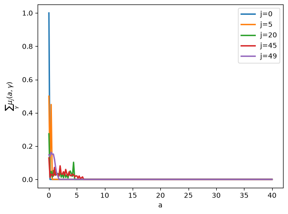
Fig. 122.1 Marginal distribution of assets by age#
A grid that is too narrow would distort these distributions by piling probability mass on the highest asset level.
Let’s verify that this does not happen here.
top_mass = μ.reshape((hh.j_grid.size, hh.a_grid.size,
                      hh.γ_grid.size))[:, -1, :].sum() / hh.j_grid.size
print(f"population share at a_max = {hh.a_grid[-1]:.0f}: {top_mass:.3%}")
population share at a_max = 40: 0.000%
Exercise 122.1 asks what happens when the upper bound binds.
These marginal distributions confirm that new agents enter the economy with no asset holdings.
the blue \(j=0\) distribution has mass only at \(a=0\).
As agents age, at first they gradually accumulate assets.
the orange \(j=5\) distribution puts positive mass on positive but low asset levels
the green \(j=20\) distribution puts positive mass on a much wider range of asset levels.
the red \(j=45\) distribution is even wider
At a later age, they gradually deplete their asset holdings.
the purple \(j=49\) distribution illustrates this
At the end of life, they will have drawn down all of their assets.
Let’s now look at age-specific optimal saving policies that generate the preceding marginal distributions of assets at different ages.
We’ll plot some saving functions with the following Python code.
σ_reshaped = σ.reshape(hh.j_grid.size, hh.a_grid.size, hh.γ_grid.size)
j_labels = [f'j={j}' for j in [0, 5, 20, 45, 49]]

fig, axs = plt.subplots(1, 2, figsize=(14, 5))

axs[0].plot(hh.a_grid, hh.a_grid[σ_reshaped[[0, 5, 20, 45, 49], :, 0].T], lw=2)
axs[0].plot(hh.a_grid, hh.a_grid, '--')
axs[0].set_xlabel("$a_{j}$")
axs[0].set_ylabel("$a^*_{j+1}$")
axs[0].legend(j_labels+['45 degree line'])
axs[0].set_title(r"Optimal saving policy, low $\gamma$")

axs[1].plot(hh.a_grid, hh.a_grid[σ_reshaped[[0, 5, 20, 45, 49], :, 1].T], lw=2)
axs[1].plot(hh.a_grid, hh.a_grid, '--')
axs[1].set_xlabel("$a_{j}$")
axs[1].set_ylabel("$a^*_{j+1}$")
axs[1].legend(j_labels+['45 degree line'])
axs[1].set_title(r"Optimal saving policy, high $\gamma$")

plt.show()
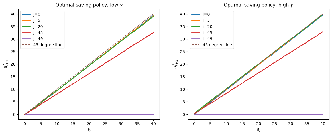
Fig. 122.2 Optimal saving policies by age#
From an implied stationary population distribution, we can compute the aggregate labor supply \(L\) and private savings \(A\).
@jax.jit
def compute_aggregates(μ, household):

    j_grid, a_grid, γ_grid, Π, β, init_μ, VJ = household

    J, a_size, γ_size = j_grid.size, a_grid.size, γ_grid.size

    μ = μ.reshape((J, household.a_grid.size, household.γ_grid.size))

    # Compute private savings
    a = a_grid.reshape((1, a_size, 1))
    A = (a * μ).sum() / J

    γ = γ_grid.reshape((1, 1, γ_size))
    lj = l(j_grid).reshape((J, 1, 1))
    L = (lj * γ * μ).sum() / J

    return A, L
A, L = compute_aggregates(μ, hh)
A, L
(Array(1.8474663, dtype=float32), Array(1.0781993, dtype=float32))
The capital stock in this economy equals \(A-D\).
D = 0
K = A - D
The firm’s optimality conditions imply interest rate \(r\) and wage rate \(w\).
KL_to_r(K, L, firm), KL_to_w(K, L, firm)
(Array(0.20578183, dtype=float32), Array(0.82273746, dtype=float32))
The implied prices \((r,w)\) differ from our guesses, so we must update our guesses and iterate until we find a fixed point.
This is our outer loop.
@jax.jit
def find_ss(household, firm, pol_target, Q, tol=1e-6, max_iter=200):

    j_grid, a_grid, γ_grid, Π, β, init_μ, VJ = household
    J = j_grid.size
    num_state = a_grid.size * γ_grid.size

    D, G, δ = pol_target

    # Initial guesses of prices
    r, w = 0.05, 1.

    # Initial guess of τ
    τ = 0.15

    def cond_fn(state):
        "The convergence criteria."

        V, σ, μ, K, L, r, w, τ, D, G, δ, r_old, w_old, i = state

        error = (r - r_old) ** 2 + (w - w_old) ** 2

        return (error > tol) & (i < max_iter)

    def body_fn(state):
        "The main body of iteration."

        V, σ, μ, K, L, r, w, τ, D, G, δ, r_old, w_old, i = state
        r_old, w_old = r, w

        # Household optimal decisions and values
        V, σ = backwards_opt([r, w], [τ, δ], household, Q)

        # Compute the stationary distribution
        μ = popu_dist(σ, household, Q)

        # Compute aggregates
        A, L = compute_aggregates(μ, household)
        K = A - D

        # Update prices
        r, w = KL_to_r(K, L, firm), KL_to_w(K, L, firm)

        # Find τ
        D_next = D
        τ = find_τ([D, D_next, G, δ],
                   [r, w],
                   [K, L])

        r = (r + r_old) / 2
        w = (w + w_old) / 2

        return V, σ, μ, K, L, r, w, τ, D, G, δ, r_old, w_old, i + 1

    # Initial state
    V = jnp.empty((J, num_state), dtype=float)
    σ = jnp.empty((J, num_state), dtype=int)
    μ = jnp.empty((J, num_state), dtype=float)

    K, L = 1., 1.
    initial_state = (V, σ, μ, K, L, r, w, τ, D, G, δ, r-1, w-1, 0)
    V, σ, μ, K, L, r, w, τ, D, G, δ, _, _, i = jax.lax.while_loop(
                                    cond_fn, body_fn, initial_state)

    # i equals max_iter if the loop stopped before converging
    return V, σ, μ, K, L, r, w, τ, D, G, δ, i
ss1 = find_ss(hh, firm, [0, 0.1, np.zeros(hh.j_grid.size)], Q)

print(f"iterations used: {ss1[-1]}")
iterations used: 10
Let’s time the computation
%time find_ss(hh, firm, [0, 0.1, np.zeros(hh.j_grid.size)], Q)[0].block_until_ready();
CPU times: user 279 ms, sys: 0 ns, total: 279 ms
Wall time: 277 ms
hh_out_ss1 = ss1[:3]
quant_ss1 = ss1[3:5]
price_ss1 = ss1[5:7]
policy_ss1 = ss1[7:11]
# V, σ, μ
V_ss1, σ_ss1, μ_ss1 = hh_out_ss1
# K, L
K_ss1, L_ss1 = quant_ss1

K_ss1, L_ss1
(Array(9.524267, dtype=float32), Array(1.0781993, dtype=float32))
# r, w
r_ss1, w_ss1 = price_ss1

r_ss1, w_ss1
(Array(0.06527545, dtype=float32), Array(1.3466222, dtype=float32))
# τ, D, G, δ
τ_ss1, D_ss1, G_ss1, δ_ss1 = policy_ss1

τ_ss1, D_ss1, G_ss1, δ_ss1
(Array(0.04824599, dtype=float32),
 Array(0, dtype=int32, weak_type=True),
 Array(0.1, dtype=float32, weak_type=True),
 Array([0., 0., 0., 0., 0., 0., 0., 0., 0., 0., 0., 0., 0., 0., 0., 0., 0.,
        0., 0., 0., 0., 0., 0., 0., 0., 0., 0., 0., 0., 0., 0., 0., 0., 0.,
        0., 0., 0., 0., 0., 0., 0., 0., 0., 0., 0., 0., 0., 0., 0., 0.],      dtype=float32))
122.12. Transition dynamics#
We compute transition dynamics using a function path_iteration.
In an outer loop, we iterate over guesses of prices and taxes.
In an inner loop, we compute the optimal consumption and saving choices by each cohort \(j\) in each time \(t\), then find the implied evolution of the joint distribution of assets and productivities.
We then update our guesses of prices and taxes given the aggregate labor supply and capital stock in the economy.
We use solve_backwards to solve for optimal saving choices given price and tax sequences and simulate_forward to compute the evolution of the joint distributions.
We require two steady states as inputs: the initial steady state to provide the initial condition for simulate_forward, and the final steady state to provide continuation values for solve_backwards.
@jax.jit
def bellman_operator(prices, taxes, V_next, household, Q):

    r, w = prices
    τ, δ = taxes

    j_grid, a_grid, γ_grid, Π, β, init_μ, VJ = household
    J = j_grid.size

    num_state = a_grid.size * γ_grid.size
    num_action = a_grid.size

    def bellman_operator_j(j):
        Rj = populate_R(j, r, w, τ, δ, household)
        vals = Rj + β * Q.dot(V_next[j+1])
        σ_j = jnp.argmax(vals, axis=1)
        V_j = vals[jnp.arange(num_state), σ_j]

        return V_j, σ_j

    V, σ = jax.vmap(bellman_operator_j, (0,))(jnp.arange(J-1))

    # The last life stage
    j = J-1
    Rj = populate_R(j, r, w, τ, δ, household)
    vals = Rj + β * Q.dot(VJ)
    σ = jnp.concatenate([σ, jnp.argmax(vals, axis=1)[jnp.newaxis]])
    V = jnp.concatenate([V, vals[jnp.arange(num_state), σ[j]][jnp.newaxis]])

    return V, σ
@jax.jit
def solve_backwards(V_ss2, σ_ss2, household, firm, price_seq, pol_seq, Q):

    j_grid, a_grid, γ_grid, Π, β, init_μ, VJ = household
    J = j_grid.size
    num_state = a_grid.size * γ_grid.size

    τ_seq, D_seq, G_seq, δ_seq = pol_seq
    r_seq, w_seq = price_seq

    T = r_seq.size

    def solve_backwards_t(V_next, t):

        prices = (r_seq[t], w_seq[t])
        taxes = (τ_seq[t], δ_seq[t])
        V, σ = bellman_operator(prices, taxes, V_next, household, Q)

        return V, (V,σ)

    ts = jnp.arange(T-2, -1, -1)
    init_V = V_ss2

    _, outputs = jax.lax.scan(solve_backwards_t, init_V, ts)
    V_seq, σ_seq = outputs
    V_seq = V_seq[::-1]
    σ_seq = σ_seq[::-1]

    V_seq = jnp.concatenate([V_seq, V_ss2[jnp.newaxis]])
    σ_seq = jnp.concatenate([σ_seq, σ_ss2[jnp.newaxis]])

    return V_seq, σ_seq
@jax.jit
def population_evolution(σt, μt, household, Q):

    j_grid, a_grid, γ_grid, Π, β, init_μ, VJ = household

    J = household.j_grid.size
    num_state = household.a_grid.size * household.γ_grid.size

    def population_evolution_j(j):

        Qσ = Q[jnp.arange(num_state), σt[j]]
        μ_next = μt[j] @ Qσ

        return μ_next

    μ_next = jax.vmap(population_evolution_j, (0,))(jnp.arange(J-1))
    μ_next = jnp.concatenate([init_μ[jnp.newaxis], μ_next])

    return μ_next
@jax.jit
def simulate_forwards(σ_seq, D_seq, μ_ss1, K_ss1, L_ss1, household, Q):

    j_grid, a_grid, γ_grid, Π, β, init_μ, VJ = household

    J, num_state = μ_ss1.shape

    T = σ_seq.shape[0]

    def simulate_forwards_t(μ, t):

        μ_next = population_evolution(σ_seq[t], μ, household, Q)

        A, L = compute_aggregates(μ_next, household)
        K = A - D_seq[t+1]

        return μ_next, (μ_next, K, L)

    ts = jnp.arange(T-1)
    init_μ = μ_ss1

    _, outputs = jax.lax.scan(simulate_forwards_t, init_μ, ts)
    μ_seq, K_seq, L_seq = outputs

    μ_seq = jnp.concatenate([μ_ss1[jnp.newaxis], μ_seq])
    K_seq = jnp.concatenate([K_ss1[jnp.newaxis], K_seq])
    L_seq = jnp.concatenate([L_ss1[jnp.newaxis], L_seq])

    return μ_seq, K_seq, L_seq
The following algorithm describes the path iteration procedure:
Algorithm 122.1 (AK-Aiyagari transition path algorithm)
Inputs Given initial steady state \(ss_1\), final steady state \(ss_2\), time horizon \(T\), and policy sequences \((D, G, \delta)\)
Output Compute equilibrium transition paths for value functions \(V\), policy functions \(\sigma\), distributions \(\mu\), and prices \((r, w, \tau)\)
Initialize from steady states:
\((V_1, \sigma_1, \mu_1) \leftarrow ss_1\) (Initial steady state)
\((V_2, \sigma_2, \mu_2) \leftarrow ss_2\) (Final steady state)
\((r, w, \tau) \leftarrow initialize\_prices(T)\) (Linear interpolation)
\(error \leftarrow \infty\), \(i \leftarrow 0\)
While \(error > \varepsilon\) and \(i \leq max\_iter\):
\(i \leftarrow i + 1\)
\((r_{\text{old}}, w_{\text{old}}, \tau_{\text{old}}) \leftarrow (r, w, \tau)\)
Backward induction: For \(t \in [T, 1]\):
For \(j \in [0, J-1]\) (age groups):
\(V[t,j] \leftarrow \max_{a'} \{u(c) + \beta\mathbb{E}[V[t+1,j+1]]\}\)
\(\sigma[t,j] \leftarrow \arg\max_{a'} \{u(c) + \beta\mathbb{E}[V[t+1,j+1]]\}\)
Forward simulation: For \(t \in [1, T]\):
\(\mu[t] \leftarrow \Gamma(\sigma[t], \mu[t-1])\) (Distribution evolution)
\(K[t] \leftarrow \int a \, d\mu[t] - D[t]\) (Aggregate capital)
\(L[t] \leftarrow \int l(j)\gamma \, d\mu[t]\) (Aggregate labor)
\(r[t] \leftarrow \alpha Z(K[t]/L[t])^{\alpha-1}\) (Interest rate)
\(w[t] \leftarrow (1-\alpha)Z(K[t]/L[t])^{\alpha}\) (Wage rate)
\(\tau[t] \leftarrow solve\_budget(r[t],w[t],K[t],L[t],D[t],G[t])\)
Compute convergence metric:
\(error \leftarrow \|r - r_{\text{old}}\| + \|w - w_{\text{old}}\| + \|\tau - \tau_{\text{old}}\|\)
Update prices with dampening:
\(r \leftarrow \lambda r + (1-\lambda)r_{\text{old}}\)
\(w \leftarrow \lambda w + (1-\lambda)w_{\text{old}}\)
\(\tau \leftarrow \lambda \tau + (1-\lambda)\tau_{\text{old}}\)
Return \((V, \sigma, \mu, r, w, \tau)\)
def path_iteration(ss1, ss2, pol_target, household, firm, Q, tol=1e-4,
                   max_iter=100, verbose=False):

    # Starting point: initial steady state
    V_ss1, σ_ss1, μ_ss1 = ss1[:3]
    K_ss1, L_ss1 = ss1[3:5]
    r_ss1, w_ss1 = ss1[5:7]
    τ_ss1, D_ss1, G_ss1, δ_ss1 = ss1[7:11]

    # Ending point: converging new steady state
    V_ss2, σ_ss2, μ_ss2 = ss2[:3]
    K_ss2, L_ss2 = ss2[3:5]
    r_ss2, w_ss2 = ss2[5:7]
    τ_ss2, D_ss2, G_ss2, δ_ss2 = ss2[7:11]

    # The given policies: D, G, δ
    D_seq, G_seq, δ_seq = pol_target
    T = G_seq.shape[0]

    # Initial guesses of prices
    r_seq = jnp.linspace(0, 1, T) * (r_ss2 - r_ss1) + r_ss1
    w_seq = jnp.linspace(0, 1, T) * (w_ss2 - w_ss1) + w_ss1

    # Initial guess of policy
    τ_seq = jnp.linspace(0, 1, T) * (τ_ss2 - τ_ss1) + τ_ss1

    error = 1
    num_iter = 0

    if verbose:
        fig, axs = plt.subplots(1, 3, figsize=(14, 3))
        axs[0].plot(jnp.arange(T), r_seq, lw=2)
        axs[1].plot(jnp.arange(T), w_seq, lw=2)
        axs[2].plot(jnp.arange(T), τ_seq, label=f'iter {num_iter}', lw=2)

    while (error > tol) and (num_iter < max_iter):
        # Repeat until finding the fixed point, or until max_iter

        r_old, w_old, τ_old = r_seq, w_seq, τ_seq

        pol_seq = (τ_seq, D_seq, G_seq, δ_seq)
        price_seq = (r_seq, w_seq)

        # Solve optimal policies backwards
        V_seq, σ_seq = solve_backwards(
            V_ss2, σ_ss2, household, firm, price_seq, pol_seq, Q)

        # Compute population evolution forwards
        μ_seq, K_seq, L_seq = simulate_forwards(
            σ_seq, D_seq, μ_ss1, K_ss1, L_ss1, household, Q)

        # Update prices by aggregate capital and labor supply
        r_seq = KL_to_r(K_seq, L_seq, firm)
        w_seq = KL_to_w(K_seq, L_seq, firm)

        # Find taxes that balance the government budget constraint
        τ_seq = find_τ([D_seq[:-1], D_seq[1:], G_seq, δ_seq],
                       [r_seq, w_seq],
                       [K_seq, L_seq])

        # Distance between new and old guesses
        error = jnp.sum((r_old - r_seq) ** 2) + \
                jnp.sum((w_old - w_seq) ** 2) + \
                jnp.sum((τ_old - τ_seq) ** 2)

        num_iter += 1
        if verbose:
            print(f"Iteration {num_iter:3d}: error = {error:.6e}")
            axs[0].plot(jnp.arange(T), r_seq, lw=2)
            axs[1].plot(jnp.arange(T), w_seq, lw=2)
            axs[2].plot(jnp.arange(T), τ_seq, label=f'iter {num_iter}', lw=2)

        r_seq = (r_seq + r_old) / 2
        w_seq = (w_seq + w_old) / 2
        τ_seq = (τ_seq + τ_old) / 2

    if error > tol:
        print(f"Warning: stopped at {num_iter} iterations with error {error:.2e}")

    if verbose:
        axs[0].set_xlabel('t')
        axs[1].set_xlabel('t')
        axs[2].set_xlabel('t')

        axs[0].set_title('r')
        axs[1].set_title('w')
        axs[2].set_title('τ')

        axs[2].legend(loc='center left', bbox_to_anchor=(1, 0.5))

    return V_seq, σ_seq, μ_seq, K_seq, L_seq, r_seq, w_seq, \
            τ_seq, D_seq, G_seq, δ_seq
We can now compute equilibrium transitions that are ignited by fiscal policy reforms.
122.13. Experiment 1: an immediate tax cut#
At \(t=0\), the government unexpectedly announces that it will issue debt.
From \(t=0\) to \(19\), debt \(D_{t+1}\) increases linearly for \(20\) periods, reaching the new target level \(D_{20} = D_0 + 1 = \bar{D} + 1\).
Government spending \(\bar{G}\) and transfers \(\bar{\delta}_j\) remain constant.
The debt path is the policy; the flat rate tax \(\tau_t\) is then whatever balances the government budget at each date.
At the announcement the residual tax rate drops well below its initial value, which is why we call this an immediate tax cut.
It then climbs steadily as debt accumulates, and once debt stops growing it settles permanently above its initial value, because the government must service the larger debt forever.
We want to compute the equilibrium transition path.
Our first step is to prepare appropriate policy variable arrays D_seq, G_seq, δ_seq
We’ll compute a τ_seq that balances government budgets.
T = 150

D_seq = jnp.ones(T+1) * D_ss1
D_seq = D_seq.at[:21].set(D_ss1 + jnp.linspace(0, 1, 21))
D_seq = D_seq.at[21:].set(D_seq[20])

G_seq = jnp.ones(T) * G_ss1

δ_seq = jnp.repeat(δ_ss1, T).reshape((T, δ_ss1.size))
In order to iterate the path, we need to first find its destination, which is the new steady state under the new fiscal policy.
ss2 = find_ss(hh, firm, [D_seq[-1], G_seq[-1], δ_seq[-1]], Q)
We can use path_iteration to find equilibrium transition dynamics.
Setting the key argument verbose=True tells the function path_iteration to display convergence information.
paths = path_iteration(ss1, ss2, [D_seq, G_seq, δ_seq], hh, firm, Q, verbose=True)
Iteration   1: error = 8.831175e-02
Iteration   2: error = 2.078297e-02
Iteration   3: error = 5.341858e-03
Iteration   4: error = 9.897855e-04
Iteration   5: error = 3.227252e-04
Iteration   6: error = 5.921904e-05
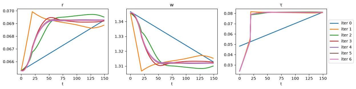
Fig. 122.3 Price path iterations for an immediate tax cut#
Having successfully computed transition dynamics, let’s study them.
V_seq, σ_seq, μ_seq = paths[:3]
K_seq, L_seq = paths[3:5]
r_seq, w_seq = paths[5:7]
τ_seq, D_seq, G_seq, δ_seq = paths[7:11]
ap = hh.a_grid[σ_seq[0]]
j = jnp.reshape(hh.j_grid, (hh.j_grid.size, 1, 1))
lj = l(j)
a = jnp.reshape(hh.a_grid, (1, hh.a_grid.size, 1))
γ = jnp.reshape(hh.γ_grid, (1, 1, hh.γ_grid.size))
t = 0

ap = hh.a_grid[σ_seq[t]]
δ = δ_seq[t].reshape((hh.j_grid.size, 1, 1))

inc = (1 + r_seq[t]*(1-τ_seq[t])) * a \
        + (1-τ_seq[t]) * w_seq[t] * lj * γ - δ
inc = inc.reshape((hh.j_grid.size, hh.a_grid.size * hh.γ_grid.size))

c = inc - ap

c_mean0 = (c * μ_seq[t]).sum(axis=1)
We care about how the policy change affects consumption across cohorts and across time.
We can study age-specific average consumption levels.
for t in [1, 10, 20, 50, 149]:

    ap = hh.a_grid[σ_seq[t]]
    δ = δ_seq[t].reshape((hh.j_grid.size, 1, 1))

    inc = (1 + r_seq[t]*(1-τ_seq[t])) * a + (1-τ_seq[t]) * w_seq[t] * lj * γ - δ
    inc = inc.reshape((hh.j_grid.size, hh.a_grid.size * hh.γ_grid.size))

    c = inc - ap

    c_mean = (c * μ_seq[t]).sum(axis=1)

    plt.plot(range(hh.j_grid.size), c_mean-c_mean0, label=f't={t}', lw=2)

plt.legend()
plt.xlabel(r'j')
plt.ylabel(r'$\Delta$ mean $C(j)$')
plt.show()
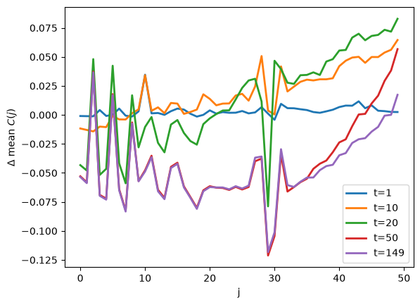
Fig. 122.4 Change in mean consumption by age#
To summarize the transition, we can plot paths as we did in Transitions in an Overlapping Generations Model.
But unlike the setup in that two-period lived overlapping generations model, we no longer have representative old and young agents.
now we have 50 cohorts of different ages at each time
To proceed, we construct two age groups of equal size – young and old.
at age 25, someone moves from being young to becoming old
ap = hh.a_grid[σ_ss1]
J = hh.j_grid.size
δ = δ_ss1.reshape((hh.j_grid.size, 1, 1))

inc = (1 + r_ss1*(1-τ_ss1)) * a + (1-τ_ss1) * w_ss1 * lj * γ - δ
inc = inc.reshape((hh.j_grid.size, hh.a_grid.size * hh.γ_grid.size))

c = inc - ap

Cy_ss1 = (c[:J//2] * μ_ss1[:J//2]).sum() / (J // 2)
Co_ss1 = (c[J//2:] * μ_ss1[J//2:]).sum() / (J // 2)
T = σ_seq.shape[0]
J = σ_seq.shape[1]

Cy_seq = np.empty(T)
Co_seq = np.empty(T)

for t in range(T):
    ap = hh.a_grid[σ_seq[t]]
    δ = δ_seq[t].reshape((hh.j_grid.size, 1, 1))

    inc = (1 + r_seq[t]*(1-τ_seq[t])) * a + (1-τ_seq[t]) * w_seq[t] * lj * γ - δ
    inc = inc.reshape((hh.j_grid.size, hh.a_grid.size * hh.γ_grid.size))

    c = inc - ap

    Cy_seq[t] = (c[:J//2] * μ_seq[t, :J//2]).sum() / (J // 2)
    Co_seq[t] = (c[J//2:] * μ_seq[t, J//2:]).sum() / (J // 2)
fig, axs = plt.subplots(3, 3, figsize=(14, 10))

# Cy (j=0-24)
axs[0, 0].plot(Cy_seq, lw=2)
axs[0, 0].hlines(Cy_ss1, 0, T, color='r', linestyle='--')
axs[0, 0].set_title('Cy (j < 25)')

# Cy (j=25-49)
axs[0, 1].plot(Co_seq, lw=2)
axs[0, 1].hlines(Co_ss1, 0, T, color='r', linestyle='--')
axs[0, 1].set_title(r'Co (j $\geq$ 25)')

names = ['K', 'L', 'r', 'w', 'τ', 'D', 'G']
for i in range(len(names)):
    i_var = i + 3
    i_axes = i + 2

    row_i = i_axes // 3
    col_i = i_axes % 3

    axs[row_i, col_i].plot(paths[i_var], lw=2)
    axs[row_i, col_i].hlines(ss1[i_var], 0, T, color='r', linestyle='--')
    axs[row_i, col_i].set_title(names[i])

# ylims
axs[1, 0].set_ylim([ss1[4]-0.1, ss1[4]+0.1])
axs[2, 2].set_ylim([ss1[9]-0.1, ss1[9]+0.1])

plt.show()
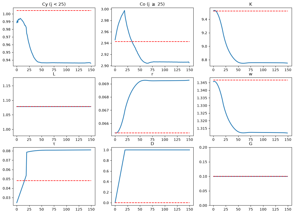
Fig. 122.5 Transition after an immediate tax cut#
Now let’s compute the mean and variance of consumption conditional on age at each time \(t\).
Cmean_seq = np.empty((T, J))
Cvar_seq = np.empty((T, J))

for t in range(T):
    ap = hh.a_grid[σ_seq[t]]
    δ = δ_seq[t].reshape((hh.j_grid.size, 1, 1))

    inc = (1 + r_seq[t]*(1-τ_seq[t])) * a + (1-τ_seq[t]) * w_seq[t] * lj * γ - δ
    inc = inc.reshape((hh.j_grid.size, hh.a_grid.size * hh.γ_grid.size))

    c = inc - ap

    Cmean_seq[t] = (c * μ_seq[t]).sum(axis=1)
    Cvar_seq[t] = ((c - Cmean_seq[t].reshape((J, 1))) ** 2 * μ_seq[t]).sum(axis=1)
J_seq, T_range = np.meshgrid(np.arange(J), np.arange(T))

fig = plt.figure(figsize=[20, 20])

# Plot the consumption mean over age and time
ax1 = fig.add_subplot(121, projection='3d')
ax1.plot_surface(T_range, J_seq, Cmean_seq, rstride=1, cstride=1,
                cmap='viridis', edgecolor='none')
ax1.set_title(r"Mean of consumption")
ax1.set_xlabel(r"t")
ax1.set_ylabel(r"j")

# plot the consumption variance over age and time
ax2 = fig.add_subplot(122, projection='3d')
ax2.plot_surface(T_range, J_seq, Cvar_seq, rstride=1, cstride=1,
                cmap='viridis', edgecolor='none')
ax2.set_title(r"Variance of consumption")
ax2.set_xlabel(r"t")
ax2.set_ylabel(r"j")

plt.show()
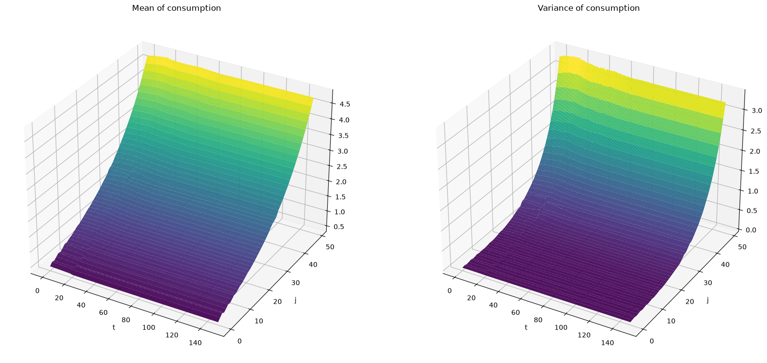
Fig. 122.6 Consumption mean and variance over age and time#
122.14. Experiment 2: a preannounced tax cut#
Now the government announces at time \(0\) that it will issue the same amount of debt, but will start doing so only after 20 periods.
As in Experiment 1, the tax rate is residual: it falls while the debt is being issued, from \(t=20\) to \(t=40\), and settles permanently above its initial level thereafter.
We will use the same key toolkit path_iteration.
We must specify D_seq appropriately.
T = 150

D_t = 20
D_seq = jnp.ones(T+1) * D_ss1
D_seq = D_seq.at[D_t:D_t+21].set(D_ss1 + jnp.linspace(0, 1, 21))
D_seq = D_seq.at[D_t+21:].set(D_seq[D_t+20])

G_seq = jnp.ones(T) * G_ss1

δ_seq = jnp.repeat(δ_ss1, T).reshape((T, δ_ss1.size))
ss2 = find_ss(hh, firm, [D_seq[-1], G_seq[-1], δ_seq[-1]], Q)
paths = path_iteration(ss1, ss2, [D_seq, G_seq, δ_seq],
                    hh, firm, Q, verbose=True)
Iteration   1: error = 5.251274e-02
Iteration   2: error = 1.731133e-02
Iteration   3: error = 3.894093e-03
Iteration   4: error = 7.399297e-04
Iteration   5: error = 2.448352e-04
Iteration   6: error = 4.188173e-05
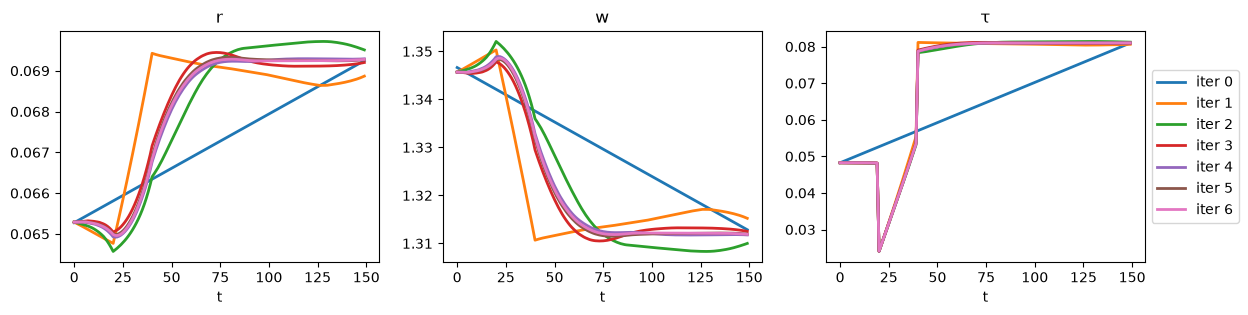
Fig. 122.7 Price path iterations for a preannounced tax cut#
V_seq, σ_seq, μ_seq = paths[:3]
K_seq, L_seq = paths[3:5]
r_seq, w_seq = paths[5:7]
τ_seq, D_seq, G_seq, δ_seq = paths[7:11]
T = σ_seq.shape[0]
J = σ_seq.shape[1]

Cy_seq = np.empty(T)
Co_seq = np.empty(T)

for t in range(T):
    ap = hh.a_grid[σ_seq[t]]
    δ = δ_seq[t].reshape((hh.j_grid.size, 1, 1))

    inc = (1 + r_seq[t]*(1-τ_seq[t])) * a + (1-τ_seq[t]) * w_seq[t] * lj * γ - δ
    inc = inc.reshape((hh.j_grid.size, hh.a_grid.size * hh.γ_grid.size))

    c = inc - ap

    Cy_seq[t] = (c[:J//2] * μ_seq[t, :J//2]).sum() / (J // 2)
    Co_seq[t] = (c[J//2:] * μ_seq[t, J//2:]).sum() / (J // 2)
Below we plot the transition paths of the economy.
fig, axs = plt.subplots(3, 3, figsize=(14, 10))

# Cy (j=0-24)
axs[0, 0].plot(Cy_seq, lw=2)
axs[0, 0].hlines(Cy_ss1, 0, T, color='r', linestyle='--')
axs[0, 0].set_title('Cy (j < 25)')

# Cy (j=25-49)
axs[0, 1].plot(Co_seq, lw=2)
axs[0, 1].hlines(Co_ss1, 0, T, color='r', linestyle='--')
axs[0, 1].set_title(r'Co (j $\geq$ 25)')

names = ['K', 'L', 'r', 'w', 'τ', 'D', 'G']
for i in range(len(names)):
    i_var = i + 3
    i_axes = i + 2

    row_i = i_axes // 3
    col_i = i_axes % 3

    axs[row_i, col_i].plot(paths[i_var], lw=2)
    axs[row_i, col_i].hlines(ss1[i_var], 0, T, color='r', linestyle='--')
    axs[row_i, col_i].set_title(names[i])

# ylims
axs[1, 0].set_ylim([ss1[4]-0.1, ss1[4]+0.1])
axs[2, 2].set_ylim([ss1[9]-0.1, ss1[9]+0.1])

plt.show()
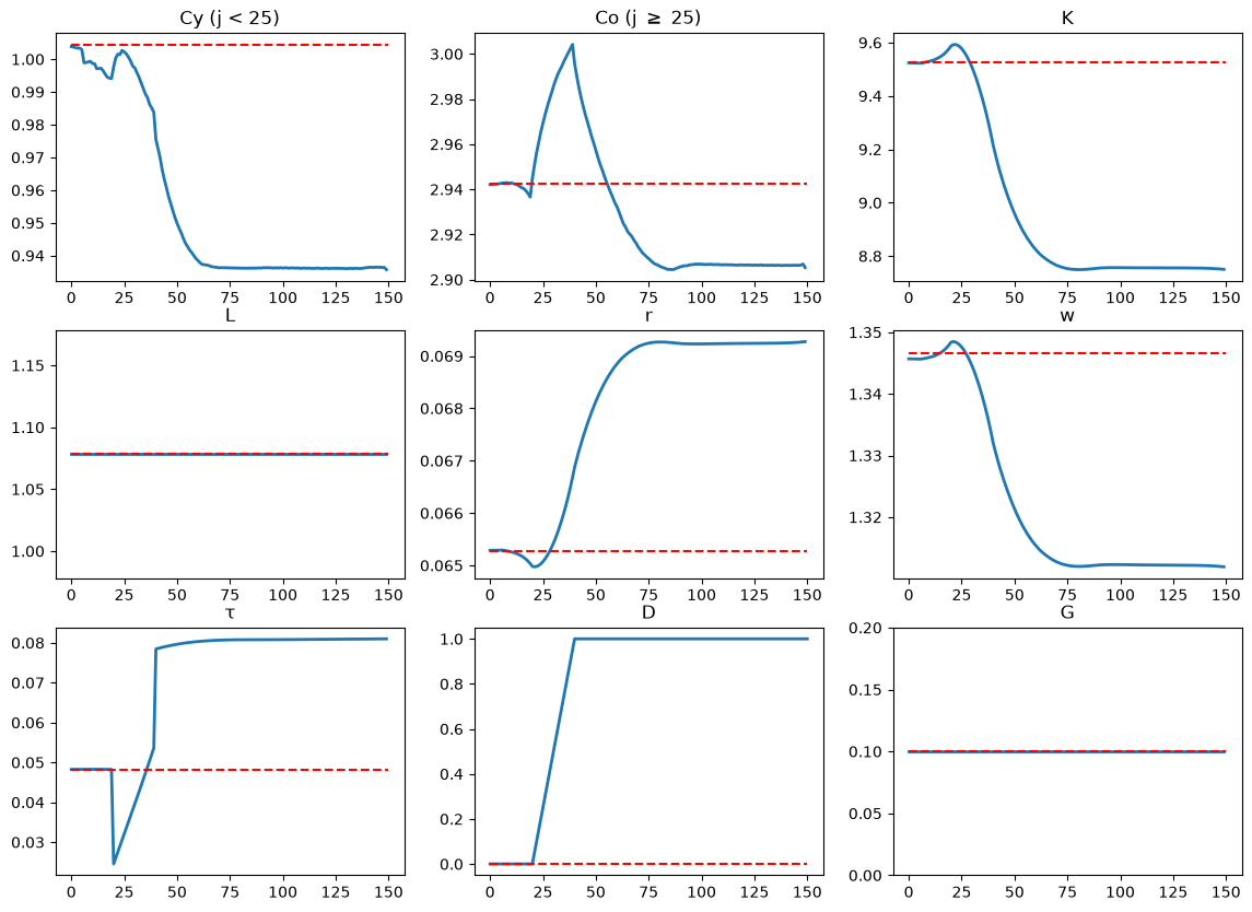
Fig. 122.8 Transition after a preannounced tax cut#
Notice how prices and quantities respond immediately, well before the policy is implemented at \(t=20\).
Agents who foresee the coming tax cut, and the permanently higher tax rate that follows it, adjust their savings right away.
Let’s zoom in on how the capital stock responds.
# K
i_var = 3
K_path = paths[i_var][:25]

K_lo = min(float(K_path.min()), float(ss1[i_var]))
K_hi = max(float(K_path.max()), float(ss1[i_var]))
pad = 0.1 * (K_hi - K_lo)

plt.plot(K_path, lw=2)
plt.hlines(ss1[i_var], 0, 25, color='r', linestyle='--')
plt.axvline(20, color='k', linestyle='--', linewidth=0.5)
plt.text(17, K_lo - 0.5 * pad, r'tax cut')
plt.ylim([K_lo - pad, K_hi + pad])
plt.ylabel("K")
plt.xlabel("t")
plt.show()
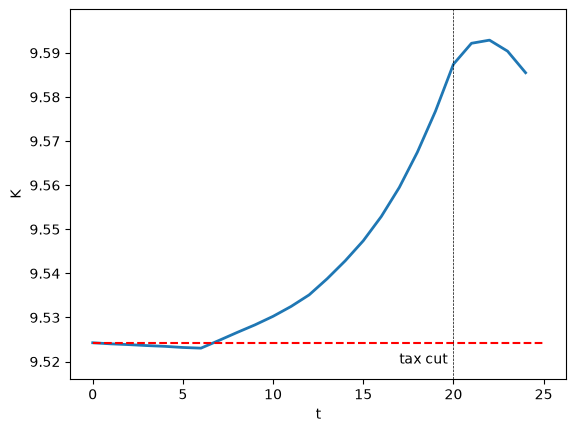
Fig. 122.9 Capital stock around the tax cut#
After the tax cut is implemented at \(t=20\), aggregate capital decreases because government debt crowds out private capital.
In the few periods just before \(t=20\), individuals save more.
The reason is that the tax cut raises the after-tax return \(r_t(1-\tau_t)\) at \(t=20\), even though the pre-tax return \(r_t\) is falling then, so saving into \(t=20\) becomes more attractive.
Because that extra saving raises the capital stock, the pre-tax interest rate dips, reaching its lowest value just before the policy takes effect.
In the first few periods after the announcement the two forces nearly cancel and the capital stock is almost flat, with the saving response building up as the implementation date approaches.
We can also plot evolutions of means and variances of consumption by different cohorts along a transition path.
Cmean_seq = np.empty((T, J))
Cvar_seq = np.empty((T, J))

for t in range(T):
    ap = hh.a_grid[σ_seq[t]]
    δ = δ_seq[t].reshape((hh.j_grid.size, 1, 1))

    inc = (1 + r_seq[t]*(1-τ_seq[t])) * a + (1-τ_seq[t]) * w_seq[t] * lj * γ - δ
    inc = inc.reshape((hh.j_grid.size, hh.a_grid.size * hh.γ_grid.size))

    c = inc - ap

    Cmean_seq[t] = (c * μ_seq[t]).sum(axis=1)
    Cvar_seq[t] = (
        (c - Cmean_seq[t].reshape((J, 1))) ** 2 * μ_seq[t]).sum(axis=1)
J_seq, T_range = np.meshgrid(np.arange(J), np.arange(T))

fig = plt.figure(figsize=[20, 20])

# Plot the consumption mean over age and time
ax1 = fig.add_subplot(121, projection='3d')
ax1.plot_surface(T_range, J_seq, Cmean_seq, rstride=1, cstride=1,
                cmap='viridis', edgecolor='none')
ax1.set_title(r"Mean of consumption")
ax1.set_xlabel(r"t")
ax1.set_ylabel(r"j")

# Plot the consumption variance over age and time
ax2 = fig.add_subplot(122, projection='3d')
ax2.plot_surface(T_range, J_seq, Cvar_seq, rstride=1, cstride=1,
                cmap='viridis', edgecolor='none')
ax2.set_title(r"Variance of consumption")
ax2.set_xlabel(r"t")
ax2.set_ylabel(r"j")

plt.show()
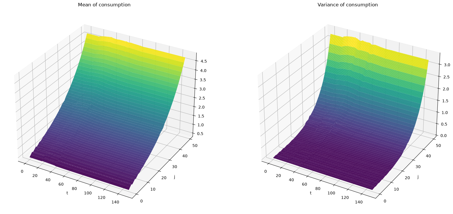
Fig. 122.10 Consumption surfaces for the preannounced tax cut#
122.15. Exercises#
Exercise 122.1
Our asset grid runs from \(0\) to \(a_{\max} = 40\).
A grid whose upper bound binds would make the computed equilibrium an artifact of the grid rather than a property of the model.
Re-solve the steady state with \(a_{\max} \in \{10, 20\}\), holding the number of grid points fixed at \(200\).
For each case report aggregate capital \(K\), the interest rate \(r\), the flat rate tax \(\tau\), and the share of the population at the top grid point.
What do you conclude about using \(a_{\max} = 10\)?
Solution
def ss_for_a_max(a_max):
    "Solve the steady state for a given upper bound on assets."
    h = create_household(a_max=a_max)
    Q_h = populate_Q(h)
    out = find_ss(h, firm, [0, 0.1, np.zeros(h.j_grid.size)], Q_h)
    μ_h = out[2].reshape((h.j_grid.size, h.a_grid.size, h.γ_grid.size))
    top = float(μ_h[:, -1, :].sum() / h.j_grid.size)
    return float(out[3]), float(out[5]), float(out[7]), top

print(f"{'a_max':>6}  {'K':>7}  {'r':>7}  {'τ':>7}  {'mass at a_max':>14}")
for a_max in [10, 20, 40]:
    K_a, r_a, τ_a, top = ss_for_a_max(a_max)
    print(f"{a_max:>6}  {K_a:>7.3f}  {r_a:>7.4f}  {τ_a:>7.4f}  {top:>13.1%}")
 a_max        K        r        τ   mass at a_max
    10    6.622   0.0843   0.0538          30.6%
    20    8.872   0.0686   0.0493           5.8%
    40    9.524   0.0653   0.0482           0.0%
With \(a_{\max} = 10\), roughly thirty percent of the population is pinned at the upper bound.
Those agents would like to hold more assets than the grid permits, so measured capital is far too low and the interest rate far too high.
Raising the bound to \(40\) empties the top of the grid and moves \(K\) up by about forty percent and \(r\) down by nearly two percentage points.
The lesson is that an upper bound must be checked, not assumed: a grid is wide enough only when almost no probability mass reaches its edge.
Exercise 122.2
How much of the capital stock is accounted for by precautionary saving against idiosyncratic labor productivity risk?
Hold the mean of \(\gamma\) at one and shrink the spread, comparing \(\gamma \in \{0.9, 1.1\}\) and \(\gamma \in \{0.75, 1.25\}\) with the baseline \(\gamma \in \{0.5, 1.5\}\).
Report \(K\), \(L\), \(r\), and \(\tau\) in each case, and explain the direction of the effect.
Solution
print(f"{'γ_grid':>16}  {'K':>7}  {'L':>7}  {'r':>7}  {'τ':>7}")
for γ_grid in [[0.9, 1.1], [0.75, 1.25], [0.5, 1.5]]:
    h = create_household(γ_grid=γ_grid)
    Q_h = populate_Q(h)
    out = find_ss(h, firm, [0, 0.1, np.zeros(h.j_grid.size)], Q_h)
    print(f"{str(γ_grid):>16}  {float(out[3]):>7.3f}  {float(out[4]):>7.4f}"
          f"  {float(out[5]):>7.4f}  {float(out[7]):>7.4f}")
          γ_grid        K        L        r        τ
      [0.9, 1.1]    9.088   1.0782   0.0674   0.0489
    [0.75, 1.25]    9.246   1.0782   0.0671   0.0487
      [0.5, 1.5]    9.524   1.0782   0.0653   0.0482
Aggregate labor \(L\) is the same in all three economies, because the productivity chain is symmetric and its mean is one in each case.
Capital nevertheless rises with the spread, from about \(9.1\) to about \(9.5\), and the interest rate falls by roughly twenty basis points.
The extra capital is precautionary saving: an agent who cannot borrow and cannot insure labor income holds a buffer stock of assets against a run of low productivity draws, and a wider spread calls for a bigger buffer.
The effect is non-linear, since most of it appears when we move from \(\{0.75, 1.25\}\) to \(\{0.5, 1.5\}\).
Note
It is tempting to shut down risk completely by setting \(\gamma_l = \gamma_h\).
Doing so is numerically treacherous.
Without idiosyncratic risk, every agent of a given age chooses the same point on the asset grid, so aggregate asset supply becomes a step function of \(r\) and the price iteration can cycle rather than converge.
This is one reason for the iteration cap in find_ss.
Exercise 122.3
This exercise builds an unfunded social security system like the one studied in Experiment 4 of the two-period model.
Let the government tax each young agent and pay each old agent, with
so that \(\sum_j \delta_j = 0\) and the scheme is balanced period by period.
Compute steady states for \(d \in \{0, 0.1, 0.25\}\) and report \(K\), \(r\), \(w\), and \(\tau\).
Report mean consumption of the young half and the old half of the population.
Compare your findings with the two-period model.
Solution
a_vec = hh.a_grid.reshape((1, hh.a_grid.size, 1))
γ_vec = hh.γ_grid.reshape((1, 1, hh.γ_grid.size))
l_vec = l(hh.j_grid).reshape((hh.j_grid.size, 1, 1))
J = hh.j_grid.size

print(f"{'d':>5}  {'K':>7}  {'r':>7}  {'w':>7}  {'τ':>7}"
      f"  {'c young':>8}  {'c old':>7}")
for d in [0.0, 0.1, 0.25]:
    δ_ss = np.zeros(J)
    δ_ss[:J//2], δ_ss[J//2:] = d, -d
    out = find_ss(hh, firm, [0, 0.1, δ_ss], Q)
    σ_d, μ_d = out[1], out[2]
    K_d, r_d, w_d, τ_d = (float(out[3]), float(out[5]),
                          float(out[6]), float(out[7]))

    ap_d = hh.a_grid[σ_d].reshape((J, hh.a_grid.size, hh.γ_grid.size))
    c_d = ((1 + r_d * (1 - τ_d)) * a_vec
           + (1 - τ_d) * w_d * l_vec * γ_vec
           - δ_ss.reshape((J, 1, 1)) - ap_d)
    c_mean = (c_d * μ_d.reshape(ap_d.shape)).sum(axis=(1, 2))

    print(f"{d:>5.2f}  {K_d:>7.3f}  {r_d:>7.4f}  {w_d:>7.4f}  {τ_d:>7.4f}"
          f"  {c_mean[:J//2].mean():>8.4f}  {c_mean[J//2:].mean():>7.4f}")
    d        K        r        w        τ   c young    c old
 0.00    9.524   0.0653   1.3466   0.0482    1.0045   2.9427
 0.10    9.212   0.0668   1.3329   0.0487    0.9212   2.9841
 0.25    8.707   0.0696   1.3103   0.0496    0.7918   3.0462
The transfer scheme is balanced at every date, so it collects no net revenue and the flat rate tax \(\tau\) barely moves.
Even so, it contracts the economy: capital falls from \(9.5\) to \(8.7\) as \(d\) rises to \(0.25\), the interest rate rises, and the wage falls.
The young consume less because they are taxed, and the old consume more because they are subsidized, but the young also save less, both because their income is lower and because the promised transfer substitutes for their own saving.
This is the same crowding out that Experiment 4 of the two-period model displays.
What the long-lived model adds is the observation that the transfer is collected from exactly those agents whose precautionary motive is strongest, namely the young, who hold the fewest assets with which to buffer labor income risk.